
California and Nevada Smoke and Air Committee
|
California and Nevada Smoke and Air Committee |
MM5 Model ConfigurationThe Penn State/NCAR Mesoscale Model 5 MM5 model employs the Lambert Conformal map projection centered at 38°N, 121°W and consists of three nested grids. The outermost grid (36 km horizontal resolution, 97x97x32 grid cells) covers the western U.S., parts of Mexico/Canada, and the eastern Pacific. The nested grid (12 km horizontal resolution, 154x154x32 grid cells) encompasses California, Nevada, Oregon, Utah, and parts of Idaho, Arizona, Wyoming, and Montana. The innermost grid (4 km horizontal resolution, 274x274x32 grid cells) encapsulates the entire California and Nevada boundaries.
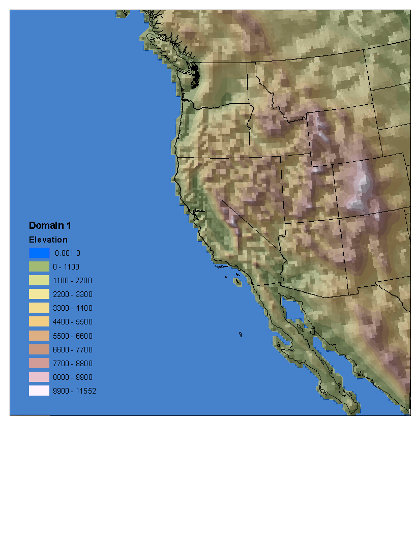
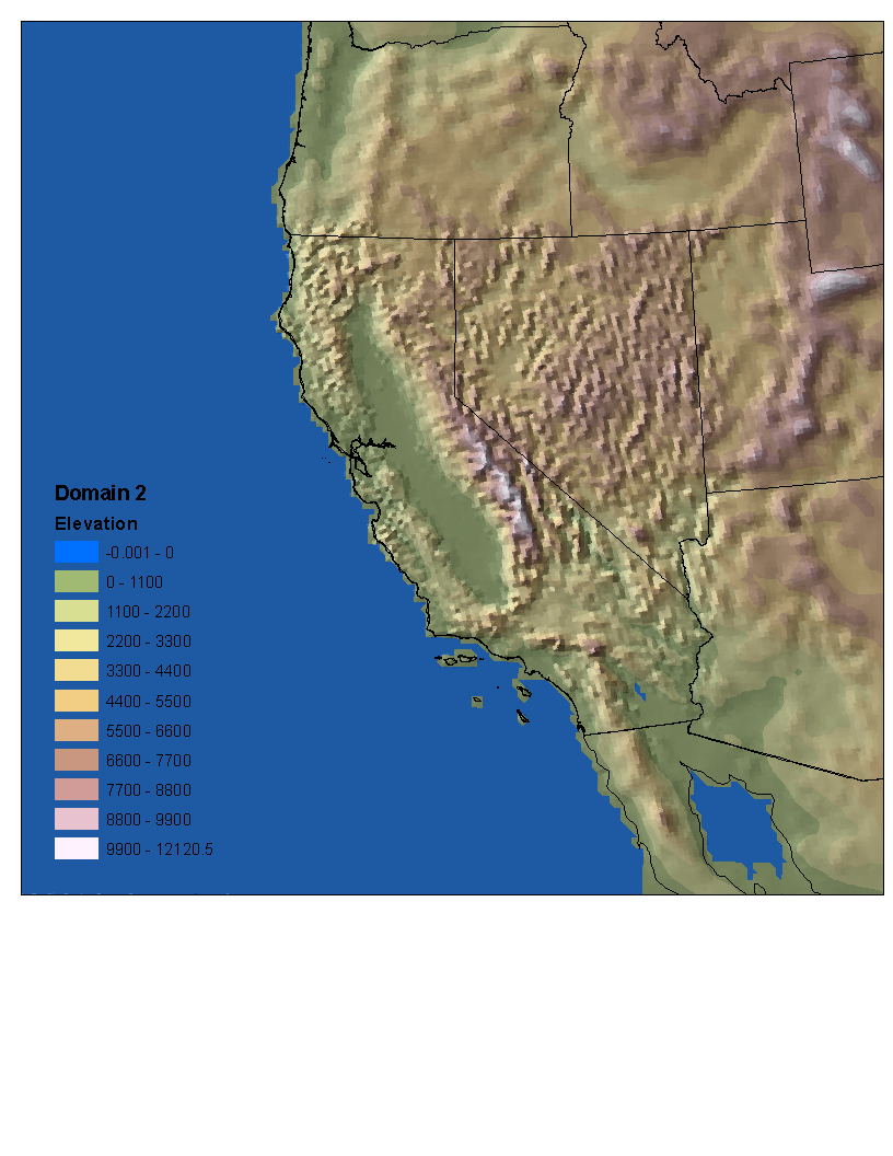
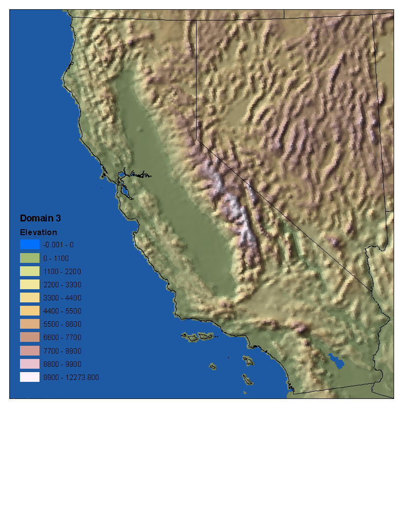
The geophysical input was derived using 10', 5' and 2' USGS terrain and land use data for the outermost, nested and innermost grids, respectively. The terrain.namelist file and the grid cell shaded relief topography figures for each domain are given here: D1 Fig, D2 Fig, D3 Fig. The corner coordinates of each grid are given in Table1. Table1. Coordinates of each model grid.
Twice daily forecasts are initialized using the National Centers for Environmental Prediction NAM model 00/12 UTC forecast outputs (Grid 212 - 40 km resolution) at 7 AM/PM PST. First guest observational fields are obtained from LDM Unidata Conduit Data Stream. Currently, the real-time system generates 72-hr forecasts for the outermost and nested grids and 48-hr forecast for the innermost grid. The model outputs are saved in 3-hourly intervals. The CANSAC real-time system utilizes the MM5 model version 3.3.6 in a non-hydrostatic mode with two-way nesting. The vertical layers consist of 32 full sigma levels for each grid (see Figure 1). The model physics options used in the current configuration are given in Table2 and the input mmlif file can be found here. Table2. The MM5 model physics options
Sigma levels:
Figure 1: This cross-section of the MM5 shows the vertical profile of the model for Domain 1 (36km horizontal resolution). The blue lines represent the vertical layers (or sigma levels) of the horizontal model grids. The model terrain is represented by the brown silhouette. Listed below is each sigma level. 1.00000, 0.99701, 0.99344, 0.98916, 0.98405, 0.97794, 0.97065, 0.96196, 0.95161, 0.93931, 0.92472, 0.90745, 0.88706, 0.86306, 0.83493, 0.80212, 0.76406, 0.72020, 0.67008, 0.61334, 0.54988, 0.47987, 0.40550, 0.33873,0.27881, 0.22501, 0.17671, 0.13336, 0.09445, 0.05951, 0.02815, 0.00000. Postprocessing The CANSAC real-time system uses the {RIP version4.0} (Read/Interpolate/Plot) visualization program with NCAR Graphics for the all post-processing products. The code is being continuously improved to meet the needs of CANSAC users. Currently the set of visual products includes plots of ventilation index, Haines index (high and mid levels), lifted index, cloud water, planetary boundary layer height, precipitation, absolute vorticity and sounding plots/text files along with other standard parameters used in weather forecasting and atmospheric assessment applications. The post-processing graphical conversion is completed in two steps with different speed and quality. After the first faster conversion (takes about half an hour) the visual products are immediately posted on the web and exchanged with the higher density products once the second and slower step is finished. This provides more timely access to the users. HardwareThe CANSAC real-time forecast system is operated on an SGI® Altix® 3700 Linux machine with 48 processors (Itanium®2 1.3 GHz) and 96 GB RAM. Currently the realtime system runs and post-processing computations are all done on the same computational environment with Intel® version7.1/8.1 compilers. The capacity of the system is composed of a 2.6 TB SGI® InfiniteStorage TP9100 Fibre Channel RAID (146 GB 10K SCSI disks) and three other 36 GB hard disks. The MM5 run takes about 1.5 hours and the entire post-processing is completed within about 2.5 hours. Benchmark results of the MM5 model run on this system can be found here. ReferencesDudhia, J., 1989. Numerical study of convection observed during the winter monsoon experiment using a mesoscale two-dimensional model. Journal of Atmospheric Sciences, 46, 3077-3107. Dudhia, J., 1996. A multi-layer soil temperature model for MM5. Preprints, The Sixth PSU/NCAR Mesoscale Model Users' Workshop, 22-24 July 1996, Boulder, Colorado, 49-50. Available online at http://www.mmm.ucar.edu/mm5/lsm/soil.pdf. Grell, A.G., Dudhia, J., Stauffer, D.R., 1995. A Description of the Fifth-Generation Penn State/NCAR Mesoscale Model (MM5). NCAR Technical Note, NCAR/TN-398 STR. National Center for Atmospheric Research, Boulder, CO. Janjic, Z.I., 1994. The step-mountain eta coordinate model: Further development of the convection, viscous sublayer, and turbulent closure schemes. Monthly Weather Review, 122, 927-945. |
||||||||||||||||||||||||||||||||